In my last post, I strongly encouraged monitoring Machine Learning (ML) models with streaming databases. In this post, I will demonstrate an example of how to do this with Materialize. If you would like to skip to the code, I have put everything in this post into AIspy, a repo on GitHub.
DTCase Study
Let’s assume that we are a machine learning practitioner who works for Down To Clown, a Direct To Consumer (DTC) company that sells clown supplies. A new user who lands on our website is called a lead. When that user purchases their first product, we say that they converted.
We built a conversion probability model to predict the probability that a lead will convert. We model this as a binary classification problem, and the outcome that we’re predicting is whether or not the lead converted.
If the conversion probability is below some threshold, then we offer the lead a coupon to entice them to convert.
What to Monitor?
For monitoring this model, at a bare minimum we would like to track standard supervised learning performance metrics such as accuracy, precision, recall, and F1 score. In practice, we should care about some metric that is better correlated with the business objective that we are trying to optimize. One of the great things about deciding to monitor your model is that it forces you to actually think about the metrics that matter and how your model exists and influences its ecosystem.
So yeah, what exactly are we trying to optimize? We probably should have thought about that when building the model, but that rarely happens.
Let’s start with money; money’s usually a good thing to maximize. In this case, we’ll focus on net revenue which is the total value of the conversion purchase minus the coupon. How does the model factor into net revenue? As with most binary classification models, it can be helpful to think through what happens in each element of the confusion matrix.
- True Positive
- The model predicts the lead will convert.
- Thus, no coupon is offered.
- The user converts.
- Net revenue is the total conversion amount.
- True Negative:
- The model thinks the lead will not convert.
- A coupon is offered.
- The lead does not convert.
- Net revenue is zero.
- False Positive:
- The model predicts the lead will convert.
- Thus, no coupon is offered.
- The lead does not convert.
- Net revenue is zero.
- False Negative:
- The model predicts the lead will not convert.
- A coupon is offered.
- The lead does convert.
- Net revenue is the total conversion amount minus the coupon amount.
Once you lay out the scenarios like this, you realize that we have an odd relationship between “standard” classification metrics and the net revenue. If we want to maximize net revenue, then we actually want to maximize the number of True Positives and False Positives. Although, if we solely maximized False Positives by offering a coupon to everybody, then we could actually have less net revenue than if we had not had any model or coupon at all, depending on the size of the coupons.
Who knew coupons could be so complicated? Let’s avoid dealing with coupon causal inference and instead just run an experiment. For some small % of users, we will deliberately not offer them a coupon. This will be our control group. We can then compare the net revenue per user between the control group and the group that can receive coupons, as well as standard supervised ML metrics.
Hack Simulacra
Now that we have our fake DTC company setup, let’s build a simulation. A plausible “data producing” scenario could be:
- I have a backend service that writes leads, conversions, and coupon data to a relational database.
- Conversion predictions are sent as events by the front end to some system that drops them into a queue, such as Kafka, for downstream processing.
Assuming this scenario, we start by creating two Postgres tables to store leads and coupons.
CREATE TABLE leads (
  id                SERIAL PRIMARY KEY,
  email             TEXT NOT NULL,
  created_at        TIMESTAMP NOT NULL DEFAULT NOW(),
  converted_at      TIMESTAMP,
  conversion_amount INT
);
CREATE TABLE coupons (
  id                SERIAL PRIMARY KEY,
  created_at        TIMESTAMP NOT NULL DEFAULT NOW(),
  lead_id           INT NOT NULL,
  -- amount is in cents.
  amount            INT NOT NULL
);
When users land on our site, we create a new lead with null converted_at and conversion_amount fields. Later, if leads do convert, then we update these fields.
For predictions, we will send these directly to a RedPanda* queue as JSON events with a form like:
{
    "lead_id": 123,
    "experiment_bucket": "experiment",
    "score": 0.7,
    "label": true,
    "predicted_at": "2022-06-09T02:25:09.139888+00:00"
}
*I’m using a RedPanda queue rather than a Kafka queue since it’s easier to setup locally. FWIW, the API is the same.
What’s left now is to actually simulate all of this. I wrote a Python script to do just that, complete with delayed conversions and everything. In the interest of not having to wait days for metrics to come in, I assume that conversions happen within a 30 second window after leads are created.
Additionally, we assume that the conversion prediction model is well correlated with conversions, the threshold is 0.5, both conversion and coupon amounts are random semi-plausible values, and the showing of the coupon does increase the chance of conversion.
What about Materialize?
What about Materialize? How about – what even is Materialize?
Let’s think back to what we want to calculate: net revenue for both the control group and the “experimental” group that is eligible for coupons, as well as standard supervised ML metrics. We would also probably want to calculate these metrics in relation to time in some way. Model metrics are necessarily aggregate functions, so we typically need to define some time window over which we will calculate them. Perhaps we want to calculate the model’s accuracy at each second for a trailing 30 second window.
Ok, so we need to calculate aggregate metrics as a function of time, and our data comes from multiple sources (Postgres + RedPanda). Materialize handles both of these requirements quite nicely.
In terms of data sources, I’ve strategically chosen data sources that play very nicely with Materialize. Very nicely. You can directly replicate Postgres tables to Materialize, and, as far as I’ve been able to tell, it just works. You can setup the replication with some SQL statements in Materialize:
CREATE MATERIALIZED SOURCE IF NOT EXISTS pg_source FROM POSTGRES
    -- Fill in with your own connection credentials.
    CONNECTION 'host=postgres user=postgres dbname=default'
    PUBLICATION 'mz_source'
    WITH (timestamp_frequency_ms = 100);

-- From that source, create views for all tables being replicated.
-- This will include the leads and coupons tables.
CREATE VIEWS FROM SOURCE pg_source;
Connecting to the RedPanda queue is not too bad either. I’m logging prediction events to a conversion_predictions topic, so you can create a view on top to convert from JSON into something like a regular, queryable SQL table:
-- Create a new source to read conversion predictions
-- from the conversion_predictions topic on RedPanda.
CREATE SOURCE IF NOT EXISTS kafka_conversion_predictions
    FROM KAFKA BROKER 'redpanda:9092' TOPIC 'conversion_predictions'
    FORMAT BYTES;

-- Conversion predictions are encoded as JSON and consumed as raw bytes.
-- We can create a view to decode this into a well typed format, making
-- it easier to use.
CREATE VIEW IF NOT EXISTS conversion_predictions AS
  SELECT
    CAST(data->>'lead_id' AS BIGINT) AS lead_id
    , CAST(data->>'experiment_bucket' AS VARCHAR(255)) AS experiment_bucket
    , CAST(data->>'predicted_at' AS TIMESTAMP) AS predicted_at
    , CAST(data->>'score' AS FLOAT) AS score
    , CAST(data->>'label' AS INT) AS label
  FROM (
    SELECT
      CONVERT_FROM(data, 'utf8')::jsonb AS data
      FROM kafka_conversion_predictions
  );
BTW, you’ll notice that my Materialize “code” is just SQL. Materialize is a database, and it follows the Postgres SQL dialect with some extra “things”.
The most important extra “thing” is the materialized view. A materialized view allows you to write a SQL query that creates something like a regular table (although it’s a view), and that “table” will stay up to date as the data changes. Whenever new data comes in (e.g. a prediction event into our RedPanda queue) or current data is updated (e.g. a lead converts), materialized views that depend on predictions or conversions will automatically be updated. While this may sound simple, and it is simple to use, ensuring that materialized views can be maintained performantly and with low latency is no trivial matter; but, Materialize does just this.
Once my data sources have been hooked into Materialize, I can then query them or create materialized views on top (and then query those views). Importantly, I can write joins between different data sources. This was one of the key requirements that I mentioned in my last post, and it’s a requirement not easily met by many modern databases.
To start, I create a non-materialized view of my conversion_predictions_dataset. This will serve as my canonical dataset of predictions joined with outcomes. This view is non-materialized which means that it gets computed on the fly when we run a query against it rather than being continuously updated and stored.
-- At each second, calculate the dataset of conversion predictions and outcomes over
-- the trailing 30 seconds.
CREATE VIEW IF NOT EXISTS conversion_prediction_dataset AS

WITH spine AS (
  SELECT
    leads.created_at AS timestamp
    , leads.id AS lead_id
  FROM leads
  WHERE
    -- The below conditions define "hopping windows" of period 2 seconds and window size
    -- 30 seconds. Basically, every 2 seconds, we are looking at a trailing 30 second
    -- window of data.
    -- See https://materialize.com/docs/sql/patterns/temporal-filters/#hopping-windows
    -- for more info
    mz_logical_timestamp() >= 2000 * (EXTRACT(EPOCH FROM leads.created_at)::bigint * 1000 / 2000)
    AND mz_logical_timestamp() < 30000 * (2000 + EXTRACT(EPOCH FROM leads.created_at)::bigint * 1000 / 2000)
)

, predictions AS (
  SELECT
    spine.lead_id
    , conversion_predictions.experiment_bucket
    , conversion_predictions.predicted_at
    , conversion_predictions.score
    , conversion_predictions.label::BOOL
  FROM spine
  LEFT JOIN conversion_predictions
    ON conversion_predictions.lead_id = spine.lead_id
)

, outcomes AS (
  SELECT
    spine.lead_id
    , CASE
        WHEN
          leads.converted_at IS NULL THEN FALSE
        WHEN
          leads.converted_at <= (leads.created_at + INTERVAL '30 seconds')
          THEN TRUE
        ELSE FALSE
      END AS value
    , CASE
        WHEN
          leads.converted_at IS NULL THEN NULL
        WHEN
          -- Make sure to only use conversion data that was known
          -- _as of_ the lead created at second.
          leads.converted_at <= (leads.created_at + INTERVAL '30 seconds')
          THEN leads.converted_at
        ELSE NULL
      END AS lead_converted_at
    , CASE
        WHEN
          leads.converted_at IS NULL THEN NULL
        WHEN
          leads.converted_at <= (leads.created_at + INTERVAL '30 seconds')
          THEN leads.conversion_amount
        ELSE NULL
      END AS conversion_amount
    , coupons.amount AS coupon_amount
  FROM spine
  LEFT JOIN leads ON leads.id = spine.lead_id
  LEFT JOIN coupons ON coupons.lead_id = spine.lead_id
)

SELECT
  date_trunc('second', spine.timestamp) AS timestamp_second
  , spine.lead_id
  , predictions.experiment_bucket
  , predictions.score AS predicted_score
  , predictions.label AS predicted_value
  , outcomes.value AS outcome_value
  , outcomes.conversion_amount
  , outcomes.coupon_amount
FROM spine
LEFT JOIN predictions ON predictions.lead_id = spine.lead_id
LEFT JOIN outcomes ON outcomes.lead_id = spine.lead_id
Finally, we get to the materialized view. For this, I use the aforementioned view to calculate model metrics at every second for a trailing 30-second window.
-- At each second, calculate the performance metrics of the
-- conversion prediction model over the trailing 30 seconds.
CREATE MATERIALIZED VIEW IF NOT EXISTS classifier_metrics AS

WITH aggregates AS (
  -- Calculate various performance metrics aggregations.
  SELECT
    timestamp_second
    , experiment_bucket
    , COUNT(DISTINCT lead_id) AS num_leads
    , SUM((predicted_value AND outcome_value)::INT)
        AS true_positives
    , SUM((predicted_value AND not outcome_value)::INT)
        AS false_positives
    , SUM((NOT predicted_value AND not outcome_value)::INT)
        AS true_negatives
    , SUM((NOT predicted_value AND not outcome_value)::INT)
        AS false_negatives
    , SUM(conversion_amount)::FLOAT / 100 AS conversion_revenue_dollars
    , (SUM(conversion_amount) - SUM(COALESCE(coupon_amount, 0)))::FLOAT / 100
        AS net_conversion_revenue_dollars
  FROM conversion_prediction_dataset
  GROUP BY 1, 2
)

-- Final metrics
SELECT
  timestamp_second
  , experiment_bucket
  , num_leads
  , true_positives
  , false_positives
  , true_negatives
  , false_negatives
  , conversion_revenue_dollars
  , net_conversion_revenue_dollars
  , true_positives::FLOAT
    / NULLIF(true_positives + false_positives, 0)
      AS precision
  , true_positives::FLOAT
    / NULLIF(true_positives + false_negatives, 0)
      AS recall
  , true_positives::FLOAT
    / NULLIF(
        true_positives
          + 1.0 / 2.0 * (false_positives + false_negatives)
        , 0
    )
      AS f1_score
FROM aggregates
Visualizing
So I have my simulation creating data in both Postgres and RedPandas, I’ve hooked these data sources into Materialize, and I’m now continually updating a materialized view of aggregate performance metrics. What do I do with this materialized view? How about a dashboard?
While perusing the Materialize demos on GitHub (which I have very liberally relied upon to create my own demo for this post), I saw that there are a number of examples that visualize materialized views with Metabase. Metabase is kind of like an open source Looker. For our purposes, we can use Metabase to create a plot of our materialized view’s fields as a function of time, and we can even setup the plot to update every second.
You see, the nice thing about using something very, conventionally database-y like Materialize is that we get to take advantage of the full ecosystem of tools that have been built around databases.
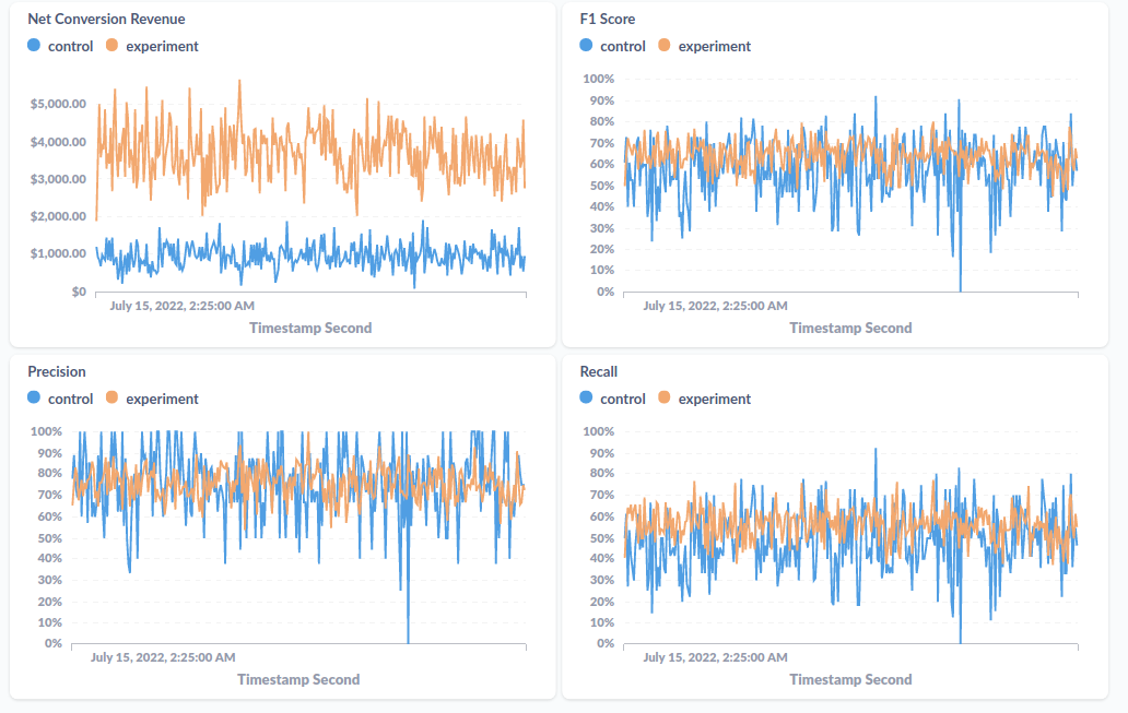
I won’t bore you with details around setting up the Metabase dashboard, but I will show you a screenshot of what this dashboard looks like for posterity:
What Next?
It’d be cool to build a lightweight framework around this. Something like:
You connect your data to Materialize and get it into a single view similar to my conversion_predictions_dataset view above. As long as you do that, the framework will build nice materialized views for standard supervised ML metrics, custom metrics, etc… along with support for slicing and dicing metrics along whatever dimensions you include.
That’s where things would start at least. The hope would be that it’s quick to get up and running, but then the more you put in, the more you get out. Send your model names and version with the predictions, and these become natural dimensions. Add support for experimentation and plugins for third party libraries. Who knows, maybe even add a feature store.
…
I would like thank Actually, nobody read this blog post before it was published, so I would not like to thank anybody. All blame rests on my shoulders.